Creating the Hero Image

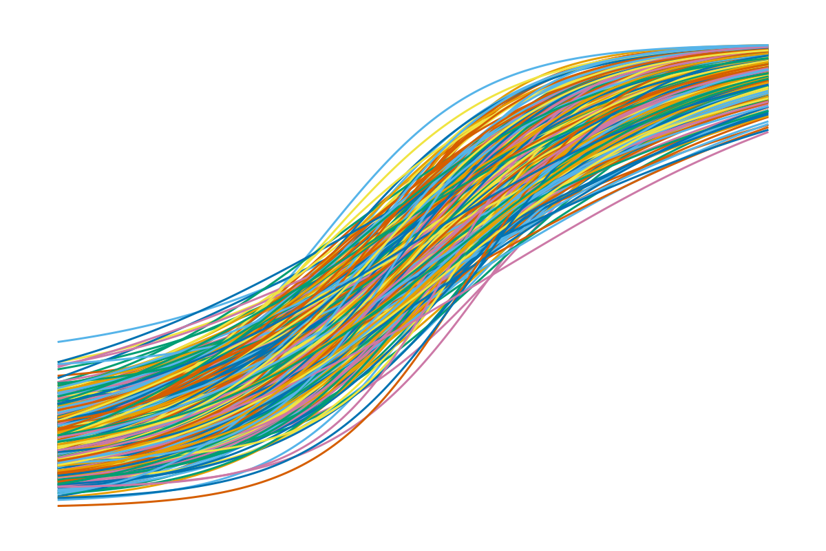
The hero image on the home page of ItemResponsePlots.jl is a random collection of item characteristic curves generated from a 3-Parameter Logistic Model. It makes use of the item_characteristic_curve! recipe.

In a first step item parameters need to be generated. The parameter distributions are chosen to yield nicely distributed curves for display.

To make the resulting plot reproducible, a random seed is set before simulation.

using Random
Random.seed!(43)

using CairoMakie
using ItemResponseFunctions
using ItemResponsePlots

n_samples = 500

items = [(
    a = exp(randn() * 0.25),
    b = randn() * 0.3,
    c = exp(randn() * 0.33 - 2.0)
) for _ in 1:n_samples]

500-element Vector{@NamedTuple{a::Float64, b::Float64, c::Float64}}:
 (a = 1.0820752074757785, b = -0.4880251296133921, c = 0.11513188957886131)
 (a = 1.2721290810761692, b = 0.34425314493992526, c = 0.10667096506196032)
 (a = 1.5979528467149198, b = -0.1804101410986923, c = 0.08167878883190725)
 (a = 1.2568272657761632, b = 0.849016232579914, c = 0.15826408139561182)
 (a = 0.8432325752602463, b = 0.16129711031252375, c = 0.35480799722516426)
 (a = 1.0068070951696275, b = 0.011004226775461484, c = 0.16148250542554002)
 (a = 1.049713974254052, b = -0.5748037955937622, c = 0.12417978409252224)
 (a = 1.159344456566031, b = -0.013244464998097314, c = 0.1578511027505735)
 (a = 1.2328113501280709, b = 0.041109469952972995, c = 0.2605516518420671)
 (a = 0.9465591237576837, b = -0.043944173031869524, c = 0.12904029268402448)
 ⋮
 (a = 0.8521473974591004, b = 0.29164341265171917, c = 0.13994763129014565)
 (a = 0.9188545343599901, b = -0.6886969150278422, c = 0.1126758290817663)
 (a = 0.6258926802994115, b = 0.7241825337045964, c = 0.08105975435162811)
 (a = 1.0196723174988027, b = 0.28541165502975435, c = 0.12438592814575933)
 (a = 1.0042937363197584, b = -0.0019721922101530276, c = 0.11443712633723174)
 (a = 1.2584415125156452, b = -0.2965248008385296, c = 0.1580829971832943)
 (a = 0.7214287238931608, b = -0.023612166925053257, c = 0.18633018495297737)
 (a = 1.2468404500187056, b = -0.061079505749674926, c = 0.11420499393233978)
 (a = 0.8956539567344826, b = 0.3245089662027561, c = 0.15360628172587867)

Once the item parameters (items) are generated, the item characteristic curves are ready to be plotted. On the most basic level this visualization just plots each item characteristic curve in a loop - the remaining code just exists to make the plot pretty! Most notably, the curves are colored by the item difficulty b.

fig = Figure()
ax = Axis(fig[1, 1])
hidedecorations!(ax)
hidespines!(ax)

normalize(x) = (x .- minimum(x)) ./ (maximum(x) - minimum(x))

colors = normalize(getindex.(items, :b))

function get_color(i)
    col = cgrad()[colors[i]]
    alpha = 0.1
    return (col, alpha)
end

thetas = -3:0.01:3

for i in eachindex(items)
    col = get_color(i)
    item_characteristic_curve!(ax, ThreePL, items[i], color = col, theta = thetas)
end

fig